Extrusion for the 3D vector view in gvSIG

As some of you might know already, some time ago we started to migrate all our tools (JGrasstools and Geopaparazzi, as well as the Nettools) to gvSIG. We are quite young in this community and we joined as an official member the gvSIG Association only at the begin of this year.

In the meanwhile we brought geopaparazzi support, the JGrasstools based Spatial Toolbox and the Epanet part of the Nettools into gvSIG.

Recently we were involved by one of the other association members, the Spanish Company DISIS, to develop with them the extrusion part for the 3D vector viewer integrated in gvSIG.

I am really thrilled by this cooperation, which brings us one more step towards the core of the community and also shows that there is movement in the gvSIG related Open Source Market.

A few notes about the extrusion plugin

From the version 2.3 of gvSIG on (well, right now the official release is not yet out), a 3d is available which allows the user to visualize layers in a Nasa World Wind 3d view. The user can select several loading modes for the layers.

The 3d properties of a vector layer can be accessed by right clicking on the layer and accessing the Properties entry in the context menu. By default the 3D tab will show up like this:

At the current time there are 3 different loading modes for vector layers:

1. Rasterized vector: the gvSIG vector layer will be rasterized as an image over the 3d view
2. Vector: the features from the gvSIG vector layer will be transformed into 3d vectors and loaded in the 3d view
3. Extruded Vector: the features from the gvSIG vector layer will be transformed into 3d vectors and loaded in the 3d view, with an applied extrusion, in order to obtain an effect of volume.

Since I have been working on the last two modes, I will give a quick insight on those.

Vector

The Vector loading mode presents the following user interface:

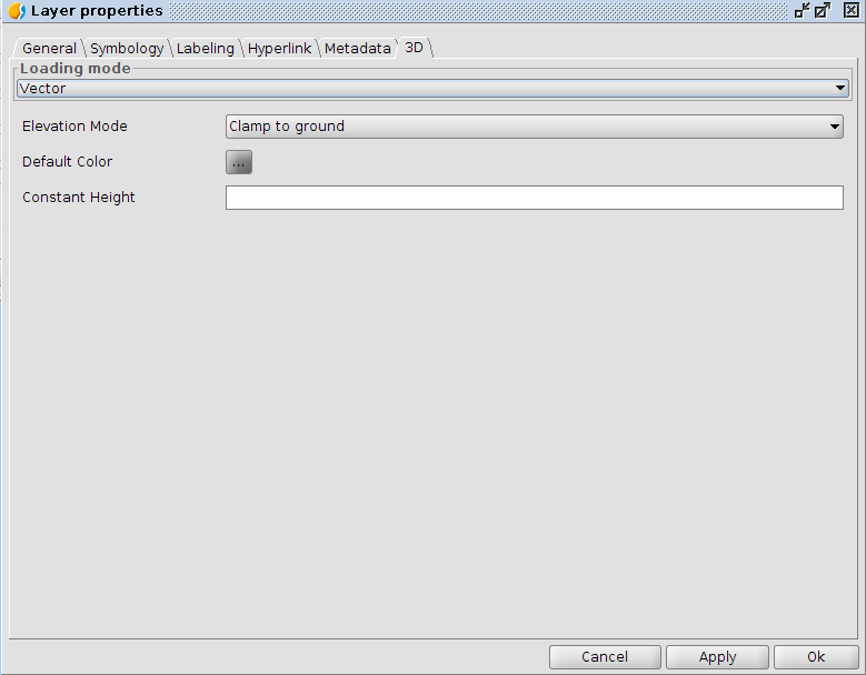
The altitude of the features can be defined by two factors (and also be the sum of both):

1. the 3rd dimension of the geometry, if available (3d shapefiles for example)
2. the Constant Height parameter

There are 3 available elevation modes, which will consider the altitude differently:

• clamp to ground: in this case the features are clamped to the elevation model currently used in the 3d view. In this case the altitude definition will not be considered.
• absolute: in this case the elevation of the vector is given by the altitude, defined as absolute elevation over the sea level.
• relative to ground: in this case the elevation of the vector is given by the altitude, defined as relative elevation over the terrain.

For example this is how the clamp to ground option would look like:
 

We can see that the very coarse default terrain model in many parts covers the vectors. In this case it is possible to set the mode to relative to ground and apply a constant height to solve it:

Extruded Vector

The extruded vector loading mode adds a couple of parameters to the user interface:
 

In this case the altitude of the features can be defined by four factors:

1. the 3rd dimension of the geometry, if available (3d shapefiles for example)
2. a Height Field from the attributes table
3. the Constant Height parameter
4. the Vertical Exaggeration, which is a multiplication factor applied to the height

There are 2 available elevation modes, which will consider the altitude differently:

• absolute: in this case the elevation of the vector is given by the altitude, defined as absolute elevation over the sea level.
• relative to ground: in this case the elevation of the vector is given by the altitude, defined as relative elevation over the terrain.

For example, if we select the relative to ground option and apply an height field that contains the building heights, this will look like:

Again we can apply a constant height to elevate the features over the terrain. Let's also try to use the number of the floors of the buildings instead of the altitude. In this cas we can apply a vertical exaggeration of 3 meters to simulate the correct building altitude:

Other examples

Example of a lines layer of isolines that have 3d coordinates. Here the extruded mode was selected and the absolute elevation mode was picked adding also a constant height of 50 additional meters:

The same layer and parameters, but without extrusion:

An example of points layer that do not have 3rd coordinates, but an absolute elevation in the attributes table. In this case the extrusion was picked and the absolute height taken from the elevation field in the attributes table:

Since the elevation is the one of the terrain, it is not possible to appreciate the extrusion effect. By adding a constant height to add as an offset, this is solved:

There is also a short video that shows 3D extrusion in gvSIG live here.

Acknowledgements

It has been great fun to implement this and also helped me know a new piece of the gvSIG internals, which is quite important right now.

So thanks to DISID for this, since our involvement in gvSIG they have always been very supportive to involve us and teach us to get up and running as fast as possible.

About 7.000.000 and more lidar points, the quest for Powerline extraction and JGrass asking help to Nasa World Wind

Do you know what this is?

More than 7.000.000 of points rendered in JGrass from a las file. Yes, It does look awsome and is well navigable (with enough ram and videocard :)).

How? By putting Nasa World Wind as a plugin into JGrass and tweak a bit the OpenGL rendering through the jogl libraries.

Why? Prototyping around extraction of powerlines.

Want to know more? What happened next?
Well... we were asked to explore a bit with feature extraction from lidar data, starting fromm the most difficult: powerlines.

While prototyping we added some tools to read las files and filter the signals through intensity, density of points, elevation difference with the dtm and things like that. Well the result up to now is pretty nice...

Ok, first let's extract the data inside a polygon... now can you see the powerlines?


Ok, let's change the coloring... no more elevation based, but intensity based:


And here we zoom in and color based on point density (in 3d), now the powerlines are already colored differently from most of the rest.



Some filtering based on intensity, density and elevation difference with the dtm and here we go (it looks empty, but have a closer look):




Let's get back to 2d using a small partial example, how does that look like?



Hmmmm, looks that one of the two is a bit wrongly placed... let's check:




Seems we are right? Check with the aerial photo:



Aha, so we are right...

Well, this is just the first part, but it already look promising.

Looking forward to mature this plugin to get it into the JGrass plugins that are going to be released.

JGrass loves Worldwind

Lately I had the need to look a bit more deep into Nasa World Wind.

With the help of the amazing examples of Patrick Murris I have been able to connect a map from a GRASS workspace to be automatically visualised and tiled for WW.

The funky thing is that while tiled, a cache is created, so it is slow only the first time.



and the same with transparency:




I am still looking for a way to substitute the elevation model of WW with a custom one on the fly.

For now this is all about prototyping and documenting, but it looks great.
Would be good to have it embeded in JGrass/uDig as its default 3D viewer?
Who knows... :)